Overview of the Python API
This is an introduction to the Python API. You will learn the basic concepts of data handling and LR calculation in LiR.
Data classes
In LiR, a dataset is represented as an InstanceData object, be it numeric features, scores, LLRs, or something else.
Specialized sub classes are:
FeatureData, for instances which has numerical features (sub class oflir.InstanceData);PairedFeatureData, for pairs of instances that have numerical features (sub class ofFeatureData);LLRData, for LLRs, with or without intervals (sub class ofFeatureData).
These objects can be instantiated manually, but in an experimental setup, they are generally provided by a
DataProvider. A DataProvider is a class that is specialized in generating, parsing or
fetching a particular type of data.
A data provider subclass implements the get_instances() method.
Example for glass data:
import numpy as np
from lir.datasets.glass import GlassData
from lir.transform.distance import ManhattanDistance
from lir.algorithms.logistic_regression import LogitCalibrator

# retrieve the data
data_provider = GlassData(cache_dir='cache')
glass_data = data_provider.get_instances()

print(f'The glass dataset has numeric features, so it is of type {type(glass_data)}.')
print(f'It has {len(glass_data)} instances, each of which is a measurement on a range of chemical elements.')

# get the number of instances for each unique source id
unique_source_ids, instance_count_by_source_id = np.unique(glass_data.source_ids, return_counts=True)
print(f'The measurements are of {len(unique_source_ids)} different sources, i.e. glass fragments.')

# get the number of sources with this many instances
instance_counts, source_counts = np.unique(instance_count_by_source_id, return_counts=True)
for instance_count, source_count in zip(instance_counts, source_counts):
    print(f'There are {source_count} sources with {instance_count} instances.')
The glass dataset has numeric features, so it is of type <class 'lir.data.models.FeatureData'>.
It has 3577 instances, each of which is a measurement on a range of chemical elements.
The measurements are of 979 different sources, i.e. glass fragments.
There are 659 sources with 3 instances.
There are 320 sources with 5 instances.
Most LR systems compare two instances, one from the trace source, and one from a reference source, and make an inference about source identity. We already acquired measurements on single glass fragments. So we pair the instances to get some pairs to compare.
from lir.transform.pairing import SourcePairing

# combine the instances into pairs
pairing_method = SourcePairing(ratio_limit=1)
pairs = pairing_method.pair(glass_data, n_ref_instances=1, n_trace_instances=1)

print(f'We have combined the {len(glass_data)} instances into {len(pairs)} pairs.')
print(f'The paired data has features of all instances in the pairs, so it has type {type(pairs)}.')
print(f'Of {len(pairs[pairs.labels==1])} pairs, both instances are from the same source.')
print(f'Of {len(pairs[pairs.labels==0])} pairs, both instances are from different sources.')
We have combined the 3577 instances into 1958 pairs.
The paired data has features of all instances in the pairs, so it has type <class 'lir.data.models.PairedFeatureData'>.
Of 979 pairs, both instances are from the same source.
Of 979 pairs, both instances are from different sources.
We have created a same-source pair for each source that has at least two instances. The number of different-source pairs
is potentially much larger, but the number of pairs created is limited to the number of same-source pairs by the
ratio_limit argument.
Some LR systems may be able to work with multiple trace and reference instances in each pair. This is relevant if there are repetitive measurements of the same source. The code below creates pairs of 2 trace instances and 3 reference instances, so we need sources with at least 5 instances for each same-source pair.
from lir.transform.pairing import SourcePairing

# combine the instances into pairs
pairing_method = SourcePairing(ratio_limit=1)
pairs_3x2 = pairing_method.pair(glass_data, n_trace_instances=2, n_ref_instances=3)

print(f'We have combined the {len(glass_data)} instances into {len(pairs_3x2)} pairs.')
print(f'The paired data has features of all instances in the pairs, so it has type {type(pairs_3x2)}.')
print(f'Of {len(pairs_3x2[pairs_3x2.labels==1])} pairs, all instances are from the same source.')
print(f'Of {len(pairs_3x2[pairs_3x2.labels==0])} pairs, the instances are from two different sources.')
We have combined the 3577 instances into 640 pairs.
The paired data has features of all instances in the pairs, so it has type <class 'lir.data.models.PairedFeatureData'>.
Of 320 pairs, all instances are from the same source.
Of 320 pairs, the instances are from two different sources.
The actual comparison can take many forms, including a distance or similarity function such as the
ManhattanDistance.
from lir.transform.distance import ManhattanDistance
from lir.algorithms.logistic_regression import LogitCalibrator

# reduce the pairs to a single value by calculating the Manhattan distance
distances = ManhattanDistance().apply(pairs)

print(f'The set of distances has type {type(distances)}.')
print(f'The distances have an average of {np.mean(distances.features)}.')
print(f'The standard deviation is {np.std(distances.features)}.')
The set of distances has type <class 'lir.data.models.FeatureData'>.
The distances have an average of 1.718129330289581.
The standard deviation is 1.8106336178949467.
Now it is time to calculate LLRs…
# calculate LLRs
llrs = LogitCalibrator().fit_apply(distances)
different_source_llrs = llrs[llrs.labels==0]
same_source_llrs = llrs[llrs.labels==1]

print(f'The set of LLRs has type {type(llrs)}.')
print(f'The median LLR for different-source pairs is {np.median(different_source_llrs.llrs)}.')
print(f'The median LLR for same-source pairs is {np.median(same_source_llrs.llrs)}.')
The set of LLRs has type <class 'lir.data.models.LLRData'>.
The median LLR for different-source pairs is -7.473422914482384.
The median LLR for same-source pairs is 1.9205078885738722.
Data strategies
Above, we training the system and calculated LLRs using the same pairs, which is not a sound experimental setup!
In an experiment we work with lir.data_strategies. This can be a simple train/test split, or a more
advanced configuration such as cross-validation.
A data strategy inherits from DataStrategy and implements an apply() method that returns an iterator
of pairs of training and test sets.
Example:
from lir.data_strategies import SourcesTrainTestSplit

splitter = SourcesTrainTestSplit(test_size=0.5)
((training_data, test_data),) = splitter.apply(glass_data)

print(f'We have {len(training_data)} instances available for training our models.')
print(f'We have {len(test_data)} instances available as test data.')
We have 1789 instances available for training our models.
We have 1788 instances available as test data.
LR systems
There can be many different LR system architectures. Refer to the selection guide if unsure which one to use.
The exact parameters depend on the type of LR system. The main ingredient is typically a pipeline of modules. The modules are executed one by one, and each module takes the output of the previous module, transforms the data, and passes the data to the next module. The modules may reduce or expand the number of features, but never change the number of instances or pairs.
An LR system may have multiple modules or pipelines as its arguments, each of which has a different role. For example, a score-based LR system has a preprocessing module, to process single instances, and a comparing module or pipeline, to calculate LLRs for the pairs.
The Pipeline class accepts any LiR module scikit-learn transformer, scikit-learn
estimator, or even other pipelines as its modules, as long as the module can work with the data.
For example, the StandardScaler transforms the data to have mean = 0 and standard deviation = 1.
Example:
from sklearn.preprocessing import StandardScaler
from lir.transform.pipeline import Pipeline

preprocessing_pipeline = Pipeline([
    ('scale', StandardScaler()),
])

normalized_glass_data = preprocessing_pipeline.fit_apply(glass_data)
A simple LR system could take the manhattan distance of each pair and then apply some kind of calibration. We can combine those steps in a pipeline.
from lir.transform.distance import ManhattanDistance
from lir.algorithms.logistic_regression import LogitCalibrator

comparing_pipeline = Pipeline([
    ('distance', ManhattanDistance()),
    ('logit', LogitCalibrator()),
])

llrs = comparing_pipeline.fit_apply(pairs)
We can use these components in a score-based LR system:
from lir.lrsystems.score_based import ScoreBasedSystem
# initialize the score-based LR system with the components we created before
lrsystem = ScoreBasedSystem(preprocessing_pipeline=preprocessing_pipeline, pairing_function=pairing_method, evaluation_pipeline=comparing_pipeline)
# use the training data to fit the LR system
lrsystem.fit(training_data)
# use the test data to calculate LLRs
llrs = lrsystem.apply(test_data)
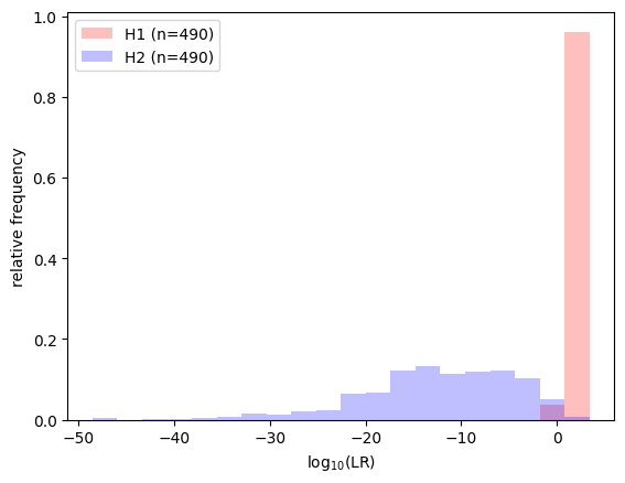
# plot results
import lir.plotting
with lir.plotting.show() as ax:
ax.lr_histogram(llrs)
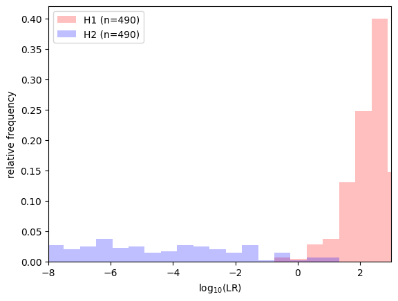
# zoom in on the LLRs around 0
with lir.plotting.show() as ax:
ax.set_xlim(-8, 3)
ax.lr_histogram(llrs, bins=100)
Above, we used a simple train/test split. Alternatives such as cross-validation use the data more efficiently, but we have to deal with multiple train/test splits.
from lir.data_strategies import SourcesCrossValidation
from lir.data.models import concatenate_instances

# initialize 5-fold cross-validation
splitter = SourcesCrossValidation(folds=5)

# initialize the results as an empty list
results = []

for training_data, test_data in splitter.apply(glass_data):
    # since we do five-fold cross-validation, we have five different
    # train/test splits of the same data

    # fitting and applying an LR system can be a one-liner
    subset_llrs = lrsystem.fit(training_data).apply(test_data)

    # add the LLRs to results list
    results.append(subset_llrs)

# combine all LLRs into a single object
llrs = concatenate_instances(*results)

# zoom in on the LLRs around 0
with lir.plotting.show() as ax:
    ax.set_xlim(-8, 3)
    ax.lr_histogram(llrs, bins=100)
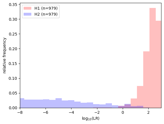
This time, we have twice as much test data altogether, because each pair appears in one of the test sets. Results should look similar compared to the train/test split.
Is this an adequate LR system?
Next step: learn how to assess an LR system’s performance.